


Insana Lab: Ultrasonic Imaging - The University of Illinois at Urbana-Champaign
Insana Lab: RF Ultrasound Data Downloads
Patient and gelatin phantom echo data from Siemens Antares™ Ultrasound System
Welcome to the downloading site for Phantom and Patient RF data. Here you will find data sets of RF
frames recorded from a gelatin phantom and 2 patients that may be downloaded. For each scanned subject
(gelatin phantom or patient) we will provide you with a simple description of the procedure, tutorial on
how to obtain a B-mode image, as well as the downloading links for the data files. These data were originally
recorded for the purpose of strain imaging and for estimation of viscoelastic features. Simply scroll down to
their respective links and double-click them.
For questions and comments, please send an email to Peggy Qiu at yqiu2@illinois.edu
DOWNLOAD MATLAB DATA 1.97 GB
Introduction to Gelatin Phantom Imaging
The phantom that we used is a block of Type B (derived from animal hide) gelatin containing graphite scatterers. The uniform properties are changed by an injection of acid which softened a region in the center of the phantom with a circular cross section. The phantom was compressed using a motion controller while being scanned by a linear array ultrasound transducer from the Antares?system. The RF echo frames are collected at a frame rate of 2-4 frames/sec.The procedure for acquiring data for viscoelastic imaging is as follows:
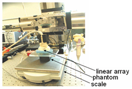
- A motion controller compresses the gel from above, as shown in Figure 1 below, as RF frames were recorded.
Figure 1: Lab setup for phantom scan
- The phantom is first compressed to a certain height using a ramp stress field, resulting in a quick increase (about 1 second) of strain so that only the elastic component of the phantom responded. This cannot be seen in Figure 2 because it is very brief. The location of this ramp response starts at t=0 and e(t)=0 and ends right where the curve in Figure 2 begins. In this case, the instantaneous elastic modulus was approximate 0.075. RF data were recorded at 4 fps for the first RF file (about 85 seconds).
- The motion controller then held the transducer assembly at a constant compression height for 25-30 minutes to allow the viscous components of the medium to respond and be recorded. RF frames were recorded at 2 fps from the 2nd RF file and onward. This can be seen in the curve in Figure 2, where the slope of the curve is becoming less steep and eventually becoming mostly linearly increasing (characteristic of phantom imaging)..
- The phantom is compressed 8% of its height. The average phantom height at rest is about 5cm.
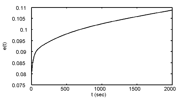
Figure 2: Stress-relaxation curve
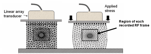
Figure 3: Pre and post compression of phantom
The following phantom data has been made available to you: It is comprised of a total of 13 RF files, each approximately 200 MB in size. Each RF file contains 343 frames, with the first RF file recorded at 4 frames/sec and all subsequent RF files recorded at 2 frames/sec.
The RF file information can be read using the URI-OPT84 program available at the URI Users Group Website. To get to the URI Users Group Website, simply look to the left column on your webpage screen and find the tab that says URI, click on that link and you will be taken to the website where you can download the software.
Each RF file is time-stamped as it recorded the last frame in the file. So that the time in-between each RF file can be calculated to match each frame when piecing all the RF frames together. You can find this information from the way that each RF file is named. For example, if you have a file named "uri_SpV1556_VpF192_FpA343_20071005151331.rfd", then the date and time this RF file is recorded (which is when all the frames of this file has been recorded) is saved as the last string of numbers in the file name: "20071005151331". This number follows the format of "YearMonthDayHourMinuteSecond". Therefore, this particular RF file is recorded at 10/05/2007 at 15:13:31. Using this information, you will be able to discern the order of the RF files in the set of 13, as well as finding out the time delay between each file recorded.
Now that we have described the process and given you some basic information about the data set available for download, you can either go back and go through the tutorial, or just click on the download link to get the RF files.
Tutorial on Gelatin Phantom Data B-mode Image Extraction and Display
The following figures are provided to show what the processed images from the provided set of RF data looks like for you to compare with your own results.
For this tutorial, we will show you how to obtain a B-mode image from the RF files. For information on how to obtain the elastogram and subsequent parametric images for the gelatin phantom, please see the following papers for reference:
The Matlab version that we have used is version R14 Service Pack 3 (Version 7.1.0.246). There are some versions of Matlab that appear to be incompatible with our URI-OPT software. Therefore, it is best to use this version in order to achieve the same results as we did.
First, let us attempt to extract and convert one RF scan to a B-mode frame. For this example we will use the very first RF file that you have downloaded (insert name of RF file here).
- Save your RF files under a folder such as C:\UltrasoundPhantomData\
- Make sure you have downloaded the aforementioned URI-OPT084 Matlab extension files, unzipped in the directory of your choice (e.g. C:\URI-OPT084\) and have set the path correctly in Matlab to access it.
- Browse through the files in the URI-OPT084 folder and find the file titled "URI2MAT.m". This is the file that will read the RF file, extract out single RF frames and output each frame as a ".mat" file.
- Start up Matlab and type in the command "URI2MAT", the following window will appear:
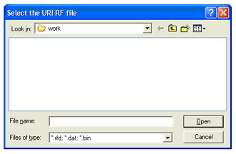
- The URI2MAT program does not specify a default file directory, so the browser will just start at whatever the
directory your Matlab is pointed to right now. Redirect the directory to where your RF files are, select the
file and click "Open". You will then see the following window:
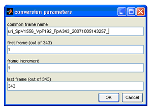
- Here is where you can set the common name for the extracted frames (e.g. all frames named starting with
"Phantom_"). Whatever name you choose to put under the "common frame name" parameter, make sure it is
followed by an "_" in order to separate the common name from the frame number that follows. Let's use
"Phantom_" as the common name. The rest of the parameters are fairly self-explanatory and usually does not
need to be changed unless you don't want to extract every frame from the RF file. In that case you will need to
change the "frame increment" parameter to the number of frames that you wish to skip every time.
For this example, we will extract every frame in the file. Your conversion parameters window should look like this now,
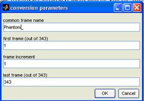
- Click "OK" and the program will start to extract and convert the RF file into single frames of RF scans. These frames will be automatically saved in the same directory as your RF files as "*.mat" files that are numbered from 1 to 343. For this example, you will see 343 files titled "Phantom_001.mat", "Phantom_002.mat" and so on until "Phantom_343.mat".
- Now that you have each RF frame extracted, I will show you how to properly display a B-mode frame in a
Matlab figure. Let's try to display the first frame as an example. In the Matlab command, enter "load('Phantom_001.mat')",
this will load the matrix into Matlab. The matrix variable is named "signals_matrix" and is a 1556x192 sized 2-D array,
note the size of the array for further calculation. This is still the RF image and an envelope detector will need to
be used to get the B-mode image back. This is done using the "log(abs(Hilbert(x)))" function in Matlab. Enter the
following command into Matlab to get the B-mode matrix, note that the dimension of the matrix is still the same
after conversion:
bm_ima=log(abs(hilbert(signals_matrix))+10);
- To display the images correctly, we will need to know its axial and lateral dimensions of the frame.
To do this, we will use the URIfileheader function included in the URI-OPT084 package to read the header
information from the RF file. Input the following commands into Matlab, when a window pops up asking for
the RF file, select the RF file that you have used to extract the "*.mat" frames.
[filename, filepath] = uigetfile('*.rfd; *.dat; *.bin', 'Select the URI RF file');
if filename == 0
return;
end
UserInput = [];
UserInput.filename = filename;
UserInput.filepath = filepath;
disp(strcat(UserInput.filepath, UserInput.filename))
clear filename filepath
FileHeader = URIfileheader(UserInput);
- You will notice that a struct file called FileHeader shows up in the workspace of Matlab.
This struct file contains all the information necessary to correctly convert the vector array into a
B-mode image. The necessary equations used to calculate the axial and lateral sizes (total length in
each direction) are:
The BmodeArray is the "bm_ima" variable that you loaded from a single frame .mat file. To find the size of a single pixel, simply divide the total length (axial or lateral) by the total number of elements in that direction (number of row or column). Double click on "FileHeader" in the workspace, then double click on the struct called "rfbm" and find the value for the variable called LineDensity. In this case, the LineDensity recorded is 50cm-1. Therefore, the axial pixel size is 0.0192mm and the lateral pixel size is 0.2mm.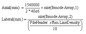
- Now we have the information to plot the B-mode image properly. First, type in the follow command to plot
the un-converted B-mode image.
figure;
Next we will need to convert the displayed scale using the following command:
imagesc(bm_ima);colormap(gray);colorbar;xlabel(strcat(num2str(round(lat_px_size*size(bm_ima,2))),' mm'));
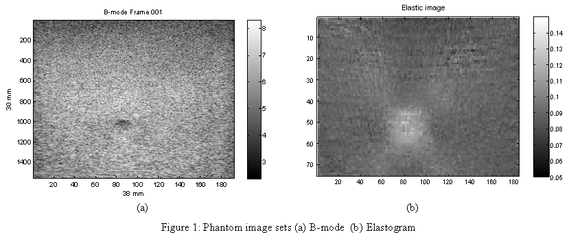
And your resultant image should look like the B-mode frame displayed in Figure 1 (a).
ylabel(strcat(num2str(round(axl_px_size*size(bm_ima,1))),' mm'));
set(gca,'plotboxaspectratio',[round(lat_px_size*size(bm_ima,2)) ...
round(axl_px_size*size(bm_ima,1)) 1])
title('B-mode Frame 001'); - The last variable that you should check is the frame rate of the data. This number can be found in the FileHeader variable. Simply double click on "FileHeader", then double click on "rfbm" and look at the variable named "AcousticFrameRateHz". In this case the frame rate is 4. This should always be checked when dealing with an unknown file because frame rate is necessary for putting the phantom strain data curve together.
NOTE: since each set of phantom data contains multiple RF files, and the URI2MAT extraction program always start the frame counting at 1, you will need to alter the code of URI2MAT in the beginning so that it a sks for a user-inputted offset that can be added to the default frame number to produce the right frame number. For example, the first RF file in the data set has frames 1 to 343, second RF file has frames 344 to 686, so the modified URI2MAT program should ask you for an offset number (which should be 343 in this case, indicated that 343 frames had already been extracted) that can be added to all the frame numbers that are being extracted from the second RF file.
For questions and comments, please send an email to Peggy Qiu at yqiu2@illinois.edu