Insana Lab: Ultrasonic Imaging - The University of Illinois at Urbana-Champaign

RF Ultrasound Data Downloads
Patient and gelatin phantom echo data from Siemens Antares™ Ultrasound System

Welcome to the downloading site for Phantom and Patient RF data. Here you will find data sets of RF frames recorded from a gelatin phantom and 2 patients that may be downloaded. For each scanned subject (gelatin phantom or patient) we will provide you with a simple description of the procedure, tutorial on how to obtain a B-mode image, as well as the downloading links for the data files. These data were originally recorded for the purpose of strain imaging and for estimation of viscoelastic features. Simply scroll down to their respective links and double-click them.

For questions and comments, please send an email to Peggy Qiu at yqiu2@illinois.edu

---

DOWNLOAD MATLAB DATA    325 MB

---

Introduction to Patient Imaging

We use a ramp-and-hold stress stimulus to initiate a creep-recovery method for imaging breast lesions. A patient lies on her side while a linear transducer array from the Antares™ System is manually pressed into the skin surface scanning in the anterior-posterior direction during a time period of approximately 15 seconds (Figure 2). The compressive force is applied within the first second and ended right where the curve in Figure 2 begins (the instantaneous elastic modulus is about 1.13), the transducer is then held in position for the rest of the scanning session. RF frames are recorded at 17 fps and a total of 12 seconds of data is available in files to be downloaded. A series of strain images is formed from adjacent RF frames using an optical flow algorithm.

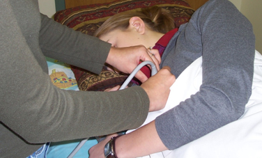
Figure 1: Patient lying on her side while an ultrasound scan is taken

A set of malignant and a set of benign patient data are available for download. Both files are from biopsy-verified studies and both presented with non-palpable tumors initially detected by mammography. Both sets provide 183 RF frames in total and are recorded at a rate of 17 frames/sec. For the malignant tumor set, the patient was diagnosed with IDC (Invasive Ductal Carcinoma). For the benign tumor set, the patient was diagnosed with fibroadenoma.

The RF file information can be read using the URI-OPT84 program available at the URI Users Group Website. To get to the URI Users Group Website, simply look to the left column on your webpage screen and find the tab that says URI, click on that link and you will be taken to the website where you can download the software.

For questions and comments, please send an email to Peggy Qiu at yqiu2@illinois.edu

---

Tutorial on Patient Data B-mode Image Extraction and Display

The following figures are provided to show what the processed images from the malignant data set look like for you to compare with your own results. The patient was diagnosed with IDC (Invasive Ductal Carcinoma).

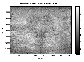
Figure 2: Figure of uncropped B-mode

The following figures are provided to show what the processed images from the benign data set look like for you to compare with your own results. The patient was diagnosed with fibroadenoma.

For this tutorial, we will show you how to obtain a B-mode image from the RF files. For information on how to obtain the elastogram and subsequent parametric images for the patient scans, please see the following papers for reference:

Pellot-Barakat C, Frouin F, Insana MF, Herment A, "Ultrasound elastography based on multi-scale estimations of displacement regularized fields," IEEE Trans. Med. Imaging 23: 153-63, 2004.

Sridhar M, Liu, J, Insana MF, "Viscoelasticity imaging using ultrasound: parameters and error analysis," Phys Med Biol, 52:2425-2443, 2007

The Matlab version that we have used is version R14 Service Pack 3 (Version 7.1.0.246). There are some versions of Matlab that appear to be incompatible with our URI-OPT software. Therefore, it is best to use this version in order to achieve the same results as we did.

First, let us attempt to extract and convert one RF scan to a B-mode frame. For this example we will use the malignant tumor RF file that you have downloaded (uri_SpV1556_VpF360_FpA183_20060307130623.rfd).

13. Save your RF files under a folder such as C:\UltrasoundPatientData\
14. Make sure you have downloaded the aforementioned URI-OPT084 Matlab extension files, unzipped in the directory of your choice (e.g. C:\URI-OPT084\) and have set the path correctly in Matlab to access it.
15. Browse through the files in the URI-OPT084 folder and find the file titled "URI2MAT.m". This is the file that will read the RF file, extract out single RF frames and output each frame as a ".mat" file.
16. Start up Matlab and type in the command "URI2MAT", the following window will appear:

    

17. The URI2MAT program does not specify a default file directory, so the browser will just start at whatever the directory your Matlab is pointed to right now. Redirect the directory to where your RF files are, select the file and click "Open". You will then see the following window:

    

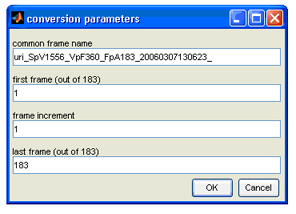
18. Here is where you can set the common name for the extracted frames (e.g. all frames named starting with "Patient_"). Whatever name you choose to put under the "common frame name" parameter, make sure it is followed by an "_" in order to separate the common name from the frame number that follows. Let's use "MalPatient_" as the common name. The rest of the parameters are fairly self-explanatory and usually does not need to be changed unless you don't want to extract every frame from the RF file. In that case you will need to change the "frame increment" parameter to the number of frames that you wish to skip every time. For this example, we will extract every frame in the file. Your conversion parameters window should look like this now,

    

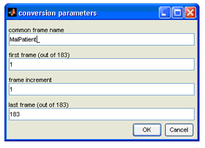
19. Click "OK" and the program will start to extract and convert the RF file into single frames of RF scans. These frames will be automatically saved in the same directory as your RF files as "*.mat" files that are numbered from 1 to 183. For this example, you will see 183 files titled "MalPatient _001.mat", "MalPatient _002.mat" and so on until "MalPatient _183.mat".
20. Now that you have each RF frame extracted, I will show you how to properly display a B-mode frame in a Matlab figure. Let's try to display the first frame as an example. In the Matlab command, enter "load('MalPatient_001.mat')", this will load the matrix into Matlab. The matrix variable is named "signals_matrix" and is a 1556x360 sized 2-D array, note the size of the array for further calculation. This is still the RF image and an envelope detector will need to be used to get the B-mode image back. This is done using the Hilbert transform function in Matlab. Enter the following command into Matlab to get the B-mode matrix, note that the dimension of the matrix is still the same after conversion:

    bm_ima=log(abs(hilbert(signals_matrix))+10);

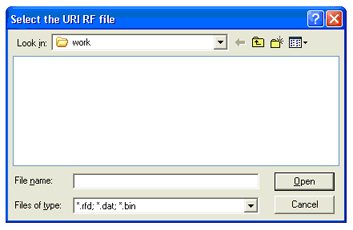
21. To display the images correctly, we will need to know its axial and lateral dimensions of the frame. To do this, we will use the URIfileheader function included in the URI-OPT084 package to read the header information from the RF file. Input the following commands into Matlab, when a window pops up asking for the RF file, select the RF file that you have used to extract the "*.mat" frames.

    [filename, filepath] = uigetfile('*.rfd; *.dat; *.bin', 'Select the URI RF file');
    if filename == 0
        return;
    end
    UserInput = [];
    UserInput.filename = filename;
    UserInput.filepath = filepath;
    disp(strcat(UserInput.filepath, UserInput.filename))
    clear filename filepath
    FileHeader = URIfileheader(UserInput);

22. You will notice that a struct file called FileHeader shows up in the workspace of Matlab. This struct file contains all the information necessary to correctly convert the vector array into a B-mode image. The necessary equations used to calculate the axial and lateral sizes (total length in each direction) are:

    

    The BmodeArray is the "bm_ima" variable that you loaded from a single frame .mat file. To find the size of a single pixel, simply divide the total length (axial or lateral) by the total number of elements in that direction (number of row or column). Double click on "FileHeader" in the workspace, then double click on the struct called "rfbm" and find the value for the variable called LineDensity. In this case, the LineDensity recorded is 93.979cm-1. Therefore, the axial pixel size is 0.0192mm and the lateral pixel size is 0.1064mm.
23. Now we have the information to plot the B-mode image properly. First, type in the follow command to plot the un-converted B-mode image. figure;

    imagesc(bm_ima);colormap(gray);colorbar;

    Next we will need to convert the displayed scale using the following command:

    xlabel(strcat(num2str(round(lat_px_size*size(bm_ima,2))),' mm'));
    ylabel(strcat(num2str(round(axl_px_size*size(bm_ima,1))),' mm'));
    set(gca,'plotboxaspectratio',[round(lat_px_size*size(bm_ima,2)) ...
    round(axl_px_size*size(bm_ima,1)) 1])
    title('Malignant Tumor Patient B-mode Frame 001');

    And your resultant image should look like the B-mode frame displayed in Figure 2.
24. In patient imaging the B-mode is cropped in order to register with sonograms. So the B-mode image titled "Registered Sonogram" is simply a smaller version of the original B-mode image. A sample registered B-mode .mat file has been provided to show you what it look like. If you follow steps 8-11 you will be able to get the image in Figure 3(a).
25. The last variable that you should check is the frame rate of the data. This number can be found in the FileHeader variable. Simply double click on "FileHeader", then double click on "rfbm" and look at the variable named "AcousticFrameRateHz". In this case the frame rate is 17.189, or roughly 17 frames/sec.

For questions and comments, please send an email to Peggy Qiu at yqiu2@illinois.edu